读取数据
#reading the images
tumor = []
path = 'D:\\data\\Tumor_detection\\archive\\brain_tumor_dataset\\yes\\*.jpg'#*表示所有
for f in glob.iglob(path):#遍历所有的yes图片
    img = cv2.imread(f)
    img = cv2.resize(img, (128, 128))#相当于reshape改变图片大小
    b, g, r = cv2.split(img)#分割为单独的通道
    img = cv2.merge([r, g, b])#改变通道顺序
    tumor.append(img)

healthy = []
path = 'D:\\data\\Tumor_detection\\archive\\brain_tumor_dataset\\no\\*.jpg'#*表示所有
for f in glob.iglob(path):#遍历所有的yes图片
    img = cv2.imread(f)
    img = cv2.resize(img, (128, 128))#类似于reshape改变图片大小
    b, g, r = cv2.split(img)#分割为单独的通道
    img = cv2.merge([r, g, b])#改变通道顺序
    healthy.append(img)

#our images
#改变数据形式
tumor = np.array(tumor, dtype=np.float32)
healthy = np.array(healthy, dtype=np.float32)
print(tumor.shape)#(154, 128, 128, 3)154表示154张图, 128 rows, 128 columns
print(healthy.shape)#(91, 128, 128, 3)91表示91张图, 128 rows, 128 columns
All = np.concatenate((healthy, tumor))
print(All.shape)#(245, 128, 128, 3)
Brain MRI 可视化
plt.imshow(healthy[0])
plt.show()
np.random.choice(5, 3)#[0, 5)中随机选3个int, e.g.[1 3 0]
def plot_random(healthy, tumor, num=5):
    #随机返回5张healthy和tumor
    healthy_imgs = healthy[np.random.choice(healthy.shape[0], 5, replace=False)]
    tumor_imgs = tumor[np.random.choice(tumor.shape[0], 5, replace=False)]

    plt.figure(figsize=(16, 9))#fix size
    #显示healthy
    for i in range(num):
        plt.subplot(1, num, i+1)
        plt.title('healthy')
        plt.imshow(healthy_imgs[i])
    # 打开显示的图片
    plt.show()
    ##显示tumor
    for i in range(num):
        plt.subplot(1, num, i+1)
        plt.title('tumor')
        plt.imshow(tumor_imgs[i])
    #打开显示的图片
    plt.show()

plot_random(healthy=healthy, tumor=tumor)
继承抽象类Dataset, Overriding getitem, len, add
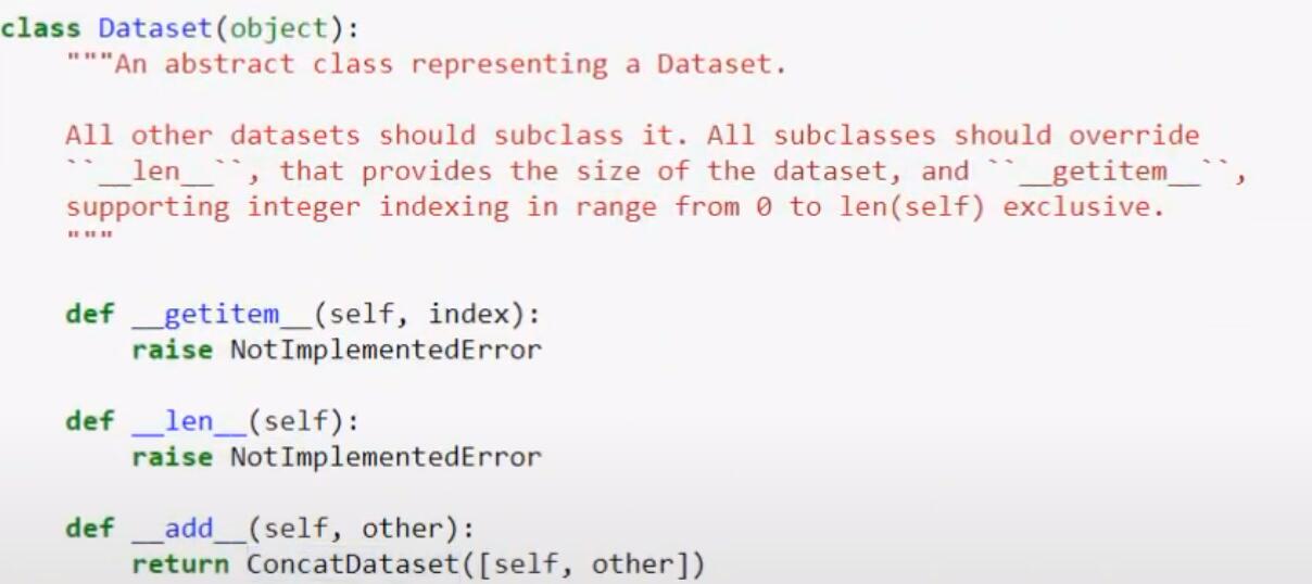
- getitem: 通过index检索数据集的特定数据
- len: 得到数据集的长度
- add: 两个数据集相加
构造一个简单的用于数组的类
class MRI(Dataset):
    def __init__(self, scores):
        self.x = scores
    def __getitem__(self, index):
        return self.x[index]
    def __len__(self):
        return len(self.x)

s1 = [1, 2, 3, 4]
d1 = MRI(s1)#s1代入构造函数中的scores
print(d1.x)#[1, 2, 3, 4]
print(d1[2])#自动调用getitem, 输出3

s2 = [100, 200, 300, 400]
d2 = MRI(s2)
#会自动调用父类中的__add__
d = d1 + d2
自定义用于MRI的dataset类
class MRI(Dataset):
    def __init__(self):
        # reading the images
        tumor = []
        path = 'D:\\data\\Tumor_detection\\archive\\brain_tumor_dataset\\yes\\*.jpg'  # *表示所有
        for f in glob.iglob(path):  # 遍历所有的yes图片
            img = cv2.imread(f)
            img = cv2.resize(img, (128, 128))  # 相当于reshape改变图片大小
            b, g, r = cv2.split(img)  # 分割为单独的通道
            img = cv2.merge([r, g, b])  # 改变通道顺序
            tumor.append(img)

        healthy = []
        path = 'D:\\data\\Tumor_detection\\archive\\brain_tumor_dataset\\no\\*.jpg'  # *表示所有
        for f in glob.iglob(path):  # 遍历所有的yes图片
            img = cv2.imread(f)
            img = cv2.resize(img, (128, 128))  # 相当于reshape改变图片大小
            b, g, r = cv2.split(img)  # 分割为单独的通道
            img = cv2.merge([r, g, b])  # 改变通道顺序
            healthy.append(img)

        # our images
        # 改变数据形式
        tumor = np.array(tumor, dtype=np.float32)
        healthy = np.array(healthy, dtype=np.float32)

        # our labels
        tumor_label = np.ones(tumor.shape[0], dtype=np.float32)  # tumor的label用1, 这里生成一堆1; tumor.shape[0]表示有多少张tumor图片
        healthy_label = np.zeros(healthy.shape[0], dtype=np.float32)  # healthy的label用0, 这里生成一堆0

        #定义实例变量; 并且连接
        #在第0轴连接: e.g.(100, 512, 512, 3)和(200, 512, 512, 3)-->(300, 512, 512, 3)最后得到300张图片[第0轴是图片数量]
        self.images = np.concatenate((tumor, healthy), axis=0)
        self.labels = np.concatenate((tumor_label, healthy_label))


    def __len__(self):
        return self.images.shape[0]#在定义类时实例变量都要加self;这里返回有多少张图
    #不仅返回image, 也要返回label; 这里返回一个包含两者的字典
    def __getitem__(self, index):


        #不仅要返回对应的图片, 也要返回label
        sample = {'image': self.images[index], 'label': self.labels[index]}
        return sample

    def normalize(self):
        self.images = self.images/255.0#255是np.max(mri)

mri = MRI()
print(len(mri))
print(mri.__getitem__(5)['image'])#打印图片的矩阵
print(mri.__getitem__(5)['image'].shape)#(128, 128, 3)宽128高128通道3
print(mri.__getitem__(5)['label'])#打印label值
DataLoader
mri = MRI()

index = list(range(len(mri)))#获取一个从0到244的list
random.shuffle(index)#打乱index元素的顺序
for idx in index:#遍历乱序的index
    sample = mri[idx]
    img = sample['image']
    label = sample['label']
    print(img.shape)
    plt.title(label)
    #只接受格式为W H C的数据
    #如果报错尝试reshape, e.g. img = img.reshape(img.shape[1], img.shape[2], img.shape[0])
    plt.imshow(img)
    plt.show()

it = iter(mri)#iter是生成迭代器的函数
for i in range(10):
    sample = next(it)#表示获取下一个包含图片以及标签的字典
    img = sample['image']
    label = sample['label']
    print(img.shape)
    plt.title(label)
    plt.imshow(img)
    plt.show()

#使用dataloader
dataloader = DataLoader(mri, batch_size=10 ,shuffle=True)
for sample in dataloader:
    img = sample["image"]
    print(img.shape)#torch.Size([10, 128, 128, 3]), 多了第一个维度为batch_size
创建一个CNN model
class CNN(nn.Module):
    def __init__(self):
        super(CNN, self).__init__()
        self.cnn_model = nn.Sequential(
            #out_channels就是过滤器/卷积核
            nn.Conv2d(in_channels=3, out_channels=6, kernel_size=5),
            nn.Tanh(),#非线性函数, 简单的数学运算
            nn.AvgPool2d(kernel_size=2, stride=5),
            #第二个卷积的通道数变为第一个的out
            nn.Conv2d(in_channels=6, out_channels=16, kernel_size=5),
            nn.Tanh(),
            nn.AvgPool2d(kernel_size=2, stride=5),
        )
        #全连接层Full Connection全连接神经网络
        self.fc_model = nn.Sequential(
            #一张128X128X3的图像经过cnn_model后得到256个值[一个矩阵]
            nn.Linear(in_features=256, out_features=120),
            nn.Tanh(),
            #上面的out_features作为下一次的in_features
            nn.Linear(in_features=120, out_features=84),
            nn.Tanh(),
            #神经网络的末端只需要一个神经元判断结果
            nn.Linear(in_features=84, out_features=1),
        )

    #向前传播, 输入的x是正确的图像
    def forward(self, x):
        x = self.cnn_model(x)
        x = x.view(x.size(0), -1)#将数据展平
        x = self.fc_model(x)
        x = F.sigmoid(x)

        return x
model = CNN()
print(model)#打印出整个神经网络的结构
print(model.cnn_model)#打印定义的cnn部分
print(model.cnn_model[0])#打印cnn第1个操作的细节:Conv2d(3, 6, kernel_size=(5, 5), stride=(1, 1))
print(model.cnn_model[0].weight)#cnn第1个操作的权重/filter/卷积核
print(model.cnn_model[0].weight.shape)#卷积核的形状:torch.Size([6, 3, 5, 5]): 6个卷积核, 3通道, 卷积核大小5X5
print(model.cnn_model[0].weight[0].shape)#第1个卷积核的形状: torch.Size([3, 5, 5])
print(model.cnn_model[0].weight[0][0])#第1个卷积核的首个通道
print(model.cnn_model[0].weight[0][2])#第1个卷积核的第2个通道
print(model.cnn_model[0].weight[0][2])#第1个卷积核的第3个通道

print(model.fc_model)#打印定义的fc_model部分
print(model.fc_model[0])#Linear(in_features=256, out_features=120, bias=True)
print(model.fc_model[0].weight.shape)#torch.Size([120, 256])


x = torch.tensor([1, 2, 3, 4, 5, 6, 7, 8, 9, 10, 11, 12, 13, 14, 15, 16])
x = x.reshape((2, 2, 2, 2))#2个数据点,2通道, 2X2的尺寸
print(x.size())#torch.Size([2, 2, 2, 2]), 打印出shape
print(x.size(0))#2, 获取第一个维度的数据, 2个数据点

print(x.view(-1))#摊平数据:tensor([ 1,  2,  3,  4,  5,  6,  7,  8,  9, 10, 11, 12, 13, 14, 15, 16])
print(x.view(x.size(0), -1))#根据第一个维度(数据点数量)摊平数据, 这里得到一个两行的矩阵 [因为有2个数据点]
在pytorch中测试一个没有训练过的新的卷积神经网络
mri_dataset = MRI()
mri_dataset.normalize()#把所有数据变成0-1之间的的
device = torch.device('cuda:0')#使用gpu计算
model = CNN().to(device)#把这个模型放入gpu

dataloader = DataLoader(mri_dataset, batch_size=32, shuffle=False)

model.eval()
outputs = []
y_true = []

with torch.no_grad():#停止梯度计算(在测试期间不计算任何梯度, 不需要计算开销和内存开销, 只是通过神经网络的数据并获得其输出)

    for D in dataloader:
        #数据默认在cpu上, 所有要使用一个to(device)
        image = D['image']
        image = image.reshape(image.shape[0], image.shape[3], image.shape[1], image.shape[2]).to(device)
        label = D['label'].to(device)

        y_hat = model(image)#y_hat存在于gpu

        #这里有32个numpy array (1 batch)
        outputs.append(y_hat.cpu().detach().numpy())
        y_true.append(y_hat.cpu().detach().numpy())

outputs = np.concatenate(outputs, axis=0).squeeze()
y_true = np.concatenate(y_true, axis=0).squeeze()

#大于0.5的被设为1[health],小于0.5的被设为0[tumor]
def threshold(scores,threshold=0.50, minimum=0, maximum = 1.0):
    x = np.array(list(scores))
    x[x >= threshold] = maximum
    x[x < threshold] = minimum
    return x

#y_true是真实的情况, threshold(outputs)是预测的情况
print(accuracy_score(y_true.round(), threshold(outputs)))#0.3714285
训练了的神经网络的效果
mri_dataset = MRI()
mri_dataset.normalize()#把所有数据变成0-1之间的的
device = torch.device('cuda:0')#使用gpu计算
model = CNN().to(device)#把这个模型放入gpu

model.eval()
outputs = []
y_true = []

eta = 0.0001#lreaning rate
EPOCH = 400
#优化器:如何在错误的表面上行走, 找到全局最小值
optimizer = torch.optim.Adam(model.parameters(), lr=eta)
dataloader = DataLoader(mri_dataset, batch_size=32, shuffle=True)
model.train()

for epoch in range(1, EPOCH):
    losses = []
    for D in dataloader:
        optimizer.zero_grad()#每一次epoc都清零优化器
        data = D['image'].to(device)
        data = data.reshape(data.shape[0], data.shape[3], data.shape[1], data.shape[2]).to(device)
        label = D['label'].to(device)
        y_hat = model(data)
        #print(y_hat.shape)#torch.Size([32, 1])
        #print(y_hat.squeeze().shape)#torch.Size([32])
        #print(label.shape)#torch.Size([32])
        # define loss function
        error = nn.BCELoss()#定义的error对象
        #将32个预测值和32个lable合起来
        loss = torch.sum(error(y_hat.squeeze(), label))
        #计算方向传播, 之后要用优化器更新数据
        loss.backward()
        optimizer.step()
        losses.append(loss.item())
    if (epoch+1) % 10 == 0:#每10个epoch打印一次avg losses
        print('Train Epoch: {}\tLoss: {:.6f}'.format(epoch+1, np.mean(losses)))

#对这个训练后的模型评估
model.eval()
dataloader = DataLoader(mri_dataset, batch_size=32, shuffle=False)
outputs = []
y_true = []
with torch.no_grad():
    for D in dataloader:
        image = D['image'].to(device)
        label = D['label'].to(device)

        image = image.reshape(image.shape[0], image.shape[3], image.shape[1], image.shape[2]).to(device)
        y_hat = model(image)

        outputs.append(y_hat.cpu().detach().numpy())
        y_true.append(label.cpu().detach().numpy())

outputs = np.concatenate(outputs, axis=0)
y_true = np.concatenate(y_true, axis=0)

#大于0.5的被设为1[health],小于0.5的被设为0[tumor]
def threshold(scores,threshold=0.50, minimum=0, maximum = 1.0):
    x = np.array(list(scores))
    x[x >= threshold] = maximum
    x[x < threshold] = minimum
    return x

#y_true是真实的情况, threshold(outputs)是预测的情况
print(accuracy_score(y_true, threshold(outputs)))#1.0